Jupyter notebook implementations can be found here
Unitary Learning without qgrad
Disclaimer: This tutorial does not use qgrad. The intention is to show follow this tutorial with another one using qgrad to show to how easier things are with qgrad.
In this tutorial, we aim to learn unitary matrices using gradient descent. The tutorial numerically reproduces part of Lloyd et al. and Bobak et al., and follows similar formalism as introduced in the two papers.
For a target unitary matrix, \(U\), we intend to find optimal parameter vectors for the parameterized unitary \(U(\vec{t}, \vec{\tau})\), such that \(U(\vec{t}, \vec{\tau})\) approximates \(U\) as closely as possible.
where \(\vec{t}\) and \(\vec{\tau}\) are parameter vectors of size \(N\) each and matrices \(A\) and \(B\) are special Hermitian matrices chosen from a Gaussian Unitary Ensemble (GUE). We shall reproduce the findings of Lloyd et al. and Bobak et al. that a \(d\) dimensional unitary can be approximated with the number of parameters \(N\) that scale as \(O(d^2)\).
For faster numerical computations we intend to learn a simple \(2 \times 2\) unitary matrix \(U\). Here the input dataset consists of \(2 \times 1\) random kets, call them \(| \psi_{l} \rangle\) and output dataset is the action of the target unitary \(U\) on these kets, \(U |\psi_{l} \rangle\). The maximum value of \(l\) is \(80\), meaning that we merely use 80 data points (kets in this case) to efficiently learn the target unitary \(U\) from \(U(\vec{t}, \vec{\tau})\)
[118]:
import matplotlib.pyplot as plt
import numpy as np
import tenpy
from qutip import fidelity, Qobj, rand_ket
from scipy.stats import unitary_group
from scipy.linalg import expm
[106]:
def make_dataset(m, d):
    r"""Prepares a dataset of input and output
        kets to be used for training.

    Args:
    ----
        m (int): Number of data points,
            80% of which would be used for training
        d (int): Dimension of a (square) unitary
            matrix to be approximated

    Returns:
    --------
        tuple: tuple of lists containing (numpy arrays of)
            input and output kets respectively.
    """
    ket_input = []
    ket_output = []
    for i in range(m):
        ket_input.append(rand_ket(d, seed=3000).full())
        #Output data -- action of unitary on a ket states
        ket_output.append(np.matmul(tar_unitr, ket_input[i]))

    return (ket_input, ket_output)


m = 100 # number of training data points
train_len = int(m * 0.8)
d = 2 #dimension of unitary
N = 4 #size of parameter vectors tau and t
# Fixed random d-dimensional target unitary matrix that we want to learn
tar_unitr = unitary_group.rvs(d)
res = make_dataset(m, d)
ket_input, ket_output = res[0], res[1]
Recipe for making \(U(\vec{t}, \vec{\tau})\)
We make \(U(\vec{t}, \vec{\tau})\) by repeated application of \(e^{-iB\tau_{k}}e^{-iAt_{k}}\) at k-th step. We multiply \(e^{-iB\tau_{k}}e^{-iAt_{k}}\) in a QAOA like fashion \(N\) times, where N is the dimension of \(\vec{t}\) and \(\vec{\tau}\). Higher N \(\rightarrow\) better approximation.
Lloyd et al. and Bobak et al., matrices \(A\) and \(B\) are chosen from a Gaussian Unitary Ensemble (GUE). We use tenpy to sample \(A\) and \(B\) from GUE.
[107]:
# tenpy for sampling A and B from GUE
A = tenpy.linalg.random_matrix.GUE((d,d))
B = tenpy.linalg.random_matrix.GUE((d,d))
[119]:
def make_unitary(N, params):
    r"""Returns a paramterized unitary matrix.

    : math:: \begin{equation}\label{decomp}
                U(\vec{t}, \vec{\tau}) =
                e^{-iB\tau_{N}}e^{-iAt_{N}} ... e^{-iB\tau_{1}}e^{-iAt_{1}}
             \end{equation}

    Args:
    ----
        N (int): Size of the parameter vectors,
            :math:`\tau` and :math:`\t`
        params (:obj:`np.ndarray`): parameter vector
                of size :math:`2 * N` where the first half
                parameters are :math:`\vec{t}` params
                and the second half encodes \vec{\tau})
                parameters.

    Returns:
        :obj:`np.ndarray`: numpy array representation of
                paramterized unitary matrix
    """
    unitary = np.eye(d)
    for i in range (N):
        unitary = np.matmul(np.matmul(
            expm(-1j * B * params[i + N][0]),
            expm(-1j * A * params[i][0])), unitary)

    return unitary
Criteria for learnability – the cost function
We use the same cost function as the authors Seth Lloyd and Reevu Maity, 2020 define
where \(|\psi_{l} \rangle\) is the input ket, \(U(\vec{t},\vec{\tau})\) and \(U\) are the parameterized and target unitaries respectively and \(M\) is the total number of training data points, which in our example is \(80\)
[109]:
def cost(params, inputs, outputs):
    r"""Calculates the cost/error on
    the whole training dataset.

    Args:
    ----
        params: parameters:math:`\t` and
            :math:`\tau` in :math:
            `U^{\dagger} U(\vec{t},\vec{\tau})`
        inputs: input kets :math:`|\psi_{l} \rangle`
            in the dataset
        outputs: output kets :math:`U(\vec{t}, \vec{\tau})
            |ket_{input}\rangle` in the dataset

    Returns:
    -------
        float: cost (evaluated on the entire
            dataset) of parametrizing
            :math:`U(\vec{t},\vec{\tau})`
            with with `params`
    """
    loss = 0.0
    for k in range(train_len):
        #prediction wth parametrized unitary
        pred = np.matmul(make_unitary(N, params), inputs[k])
        loss += np.absolute(np.real(
            np.matmul(outputs[k].conjugate().T, pred)))
    return 1 - (1 / train_len) * loss
Differentation of the cost function
Gradient descent is a first order method, so one definitely needs to take the derivative of the cost function. Analytically, the gradient of above error term, or the cost function, is
We shall, however, write a simpler derivative routine using finite differences
[110]:
def der_cost(params, inputs, outputs):
    r"""Calculates the numerical
    derivative of the cost w.r.t
    to each parameter in the cost
    function.

    Args:
        params (obj:`np.ndarray`): parameters
            :math:`\t` and :math:`\tau` in :math:
            `U^{\dagger} U(\vec{t},\vec{\tau})`
        inputs (obj:`np.ndarray`): input kets
            :math:`|\psi_{l} \rangle` in the dataset
        outputs (obj:`np.ndarray`): output kets
            :math:`U(\vec{t}, \vec{\tau})
            |ket_{input}\rangle` in the dataset

    Returns:
        :obj:`np.ndarray`: Array of cost derivatives
        w.r.t each of the parameters.

    """
    grad = []
    for i in range(params.shape[0]):
        eps = np.zeros((params.shape[0], 1))
        eps[i] = eps[i] + 1e-3
        grad.append((cost(params+eps, inputs, outputs)
                     - cost(params, inputs, outputs)) / 1e-3)
    return np.array(grad).reshape(params.shape[0], 1)
Performance Metric – Fidelity
While cost is a valid metric to judge the learnability. We introduce another commonly used metric, the average fidelity between the predicted and the output (label) states, as another metric to track during training. Average fidelity over the dataset over a particular set of parameters is defined as:
where \(\psi_{label}\) represents the resulting (or the output) ket evolved under the target unitary, \(U\) as \(U |\psi_{l} \rangle\) and \(\psi_{pred}\) represents the ket \(\psi_{l}\) evolved under \(U(\vec{t}, \vec{\tau})\) as \(U(\vec{t}, \vec{\tau})|\psi_{l} \rangle\).
[111]:
def test_score(params, x, y):
    """Calculates the average fidelity
    between the predicted and output
    kets for a given on the whole dataset.

    Args:
        params (obj:`np.ndarray`): parameters
            :math:`\t` and :math:`\tau` in :math:
            `U^{\dagger} U(\vec{t},\vec{\tau})`
        inputs (obj:`np.ndarray`): input kets
            :math:`|\psi_{l} \rangle` in the dataset
        outputs (obj:`np.ndarray`): output kets
            :math:`U(\vec{t}, \vec{\tau})
            |ket_{input}\rangle` in the dataset

       Returns:
           float: fidelity between :math:`U(\vec{t},
               \vec{\tau})|ket_{input} \rangle` and the output
               (label) kets for parameters :math:`\vec{t},
               \vec{\tau}` averaged over the entire training set.
       """
    fidel = 0
    for i in range(train_len):
        pred = np.matmul(make_unitary(N, params), x[i])
        step_fidel = fidelity(Qobj(pred), Qobj(y[i]))
        fidel += step_fidel

    return fidel / train_len
Gradient Descent Implementation
We implement gradient descent based on
for every parameter \(t_{k}\), where \(\alpha\) is the learning rate.
[120]:
np.random.seed(1000)
epochs = 15
alpha = 1e-1
loss_hist = []
fidel_hist = []
params_hist = []
weights = np.random.rand(2 * N, 1)

for epoch in range(epochs):
    weights = weights - alpha * (der_cost(weights, ket_input, ket_output))
    loss = cost(weights, ket_input, ket_output).item() # convert numpy (1,1) array to native python float
    avg_fidel = test_score(weights, ket_input, ket_output)
    progress = [epoch+1, loss, avg_fidel]
    loss_hist.append(loss)
    fidel_hist.append(avg_fidel)
    params_hist.append(weights)
    if ((epoch) % 5 == 4):
        print("Epoch: {:2f} | Loss: {:3f} | Fidelity: {:3f}".
          format(*np.asarray(progress)))
Epoch: 5.000000 | Loss: 0.092668 | Fidelity: 0.908482
Epoch: 10.000000 | Loss: 0.011956 | Fidelity: 0.988249
Epoch: 15.000000 | Loss: 0.001602 | Fidelity: 0.998427
Efficient reconstruction of the target unitary
The papers claim that if the dimension, N, of the parameters is of order \(O(d^{2})\), where \(d\) is the dimension of the unitary, then \(U(\vec{t},\vec{\tau})\) is constructed efficiently. We see how this holds true for \(d = 2\) and \(N = 4\).
[122]:
plt.figure(figsize=(9, 6))
plt.plot(range(epochs), np.asarray(fidel_hist).ravel(), marker = 'o',
         label=r"$F_{avg} = \frac{1}{M}\sum_{l}| \langle \psi_{in} | \psi_{pred} \rangle |^2$")
plt.plot( range(epochs), np.asarray(loss_hist).ravel(), marker = 'x',
        label=r"$L = 1 - (\frac{1}{M})\sum_{l}\langle \psi_{l} | U ^{\dagger} U(\vec{t},\vec{\tau}) | \psi_{l} \rangle$")
plt.title("Fidelity and Cost Trends", fontweight = "bold")
plt.legend(["Fidelity","Loss"])
plt.xlabel("epoch")
plt.legend(loc=0, prop = {'size': 15})
[122]:
<matplotlib.legend.Legend at 0x7f682646bdd8>
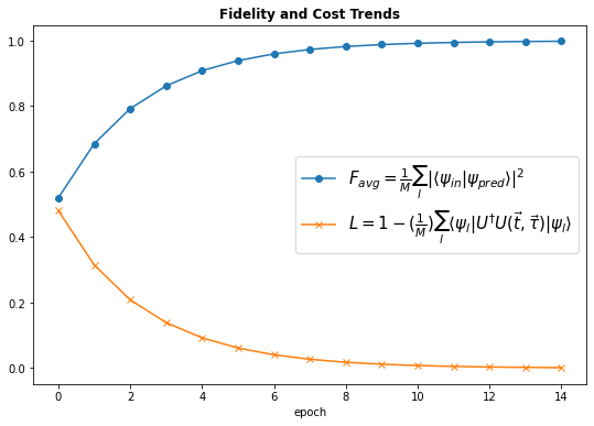
We would expect the average fidelity, \(F_{avg}\), to increase since we defined average fidelity to be between \(U(\vec{t}, \vec{\tau})|ket_{input} \rangle\) and the output (label) kets for parameters \(\vec{t}, \vec{\tau}\) at a given point in training . The expected pattern is reflected in the training graph above with the loss, \(L\), decreases progressively and the fidelity , \(F_{avg}\), increases.
Testing on unseen kets
We reserved the last \(20\) (which is \(20 \%\) of the total dataset) kets for testing. Now we shall apply our learned unitary matrix, call it \(U_{opt}(\vec{t}, \vec{\tau})\) to the unseen kets and measure the fidelity of the evolved ket under \(U_{opt}(\vec{t}, \vec{\tau})\) with those that evolved under the target unitary, \(U\).
[125]:
opt_unitary = make_unitary(N, params_hist[-1])
fidel = []
for i in range(train_len, m): # unseen data
    pred = np.matmul(opt_unitary, ket_input[i])
    fidel.append(fidelity(Qobj(pred), Qobj(ket_output[i])))
fidel
[125]:
[0.9984274341644953,
 0.9984274341644953,
 0.9984274341644953,
 0.9984274341644953,
 0.9984274341644953,
 0.9984274341644953,
 0.9984274341644953,
 0.9984274341644953,
 0.9984274341644953,
 0.9984274341644953,
 0.9984274341644953,
 0.9984274341644953,
 0.9984274341644953,
 0.9984274341644953,
 0.9984274341644953,
 0.9984274341644953,
 0.9984274341644953,
 0.9984274341644953,
 0.9984274341644953,
 0.9984274341644953]
Conclusion
The learned unitary matrix, \(U(\vec{t}, \vec{\tau})\), almost perfectly reconstructs the target unitary, \(U\), in the sense that the way \(U\) evolves a ket \(|\psi_{l} \rangle\), \(U(\vec{t}, \vec{\tau})\) also evovles \(|\psi_{l} \rangle\) in about the same way.
References
Lloyd, Seth, and Reevu Maity. “Efficient implementation of unitary transformations.” arXiv preprint arXiv:1901.03431 (2019).
Kiani, Bobak Toussi, Seth Lloyd, and Reevu Maity. “Learning unitaries by gradient descent.” arXiv preprint arXiv:2001.11897 (2020).