Jupyter notebook implementations can be found here

Learning a parametrized quantum circuit

In this tutorial, we show how qgrad can be used to perform circuit learning as well, in that how it helps us to take gradients of circuits.

For this example, we will train a simple variational quantum circuit. We shall apply rotations around \(X, Y\) and \(Z\) axes and shall use CNOT as an entangling gate. Note that qgrad was not motivated to be a circuit library, so one would have to define the gates themselves, which understandably creates some friction when working with quantum circuits. The goal of this tutorial, however, is to merely showcase that circuit learning is indeed possible in qgrad

We train a two-qubit circuit and measure the the first qubit and take the expectation with respect to the \(\sigma_{z}\) operator. This serves as our cost function in this routine and the aim is to minimize this cost function using optimal rotation angles for the rotation gates.

from functools import reduce

import jax.numpy as jnp
from jax.random import PRNGKey, uniform
from jax.experimental import optimizers
from jax import grad

from qutip import sigmaz

import matplotlib.pyplot as plt

from qgrad.qgrad_qutip import basis, expect, sigmaz, Unitary

def rx(phi):
    """Rotation around x-axis

    Args:
        phi (float): rotation angle

    Returns:
        :obj:`jnp.ndarray`: Matrix
        representing rotation around
        the x-axis

    """
    return jnp.array([[jnp.cos(phi / 2), -1j * jnp.sin(phi / 2)],
                     [-1j * jnp.sin(phi / 2), jnp.cos(phi / 2)]])

def ry(phi):
    """Rotation around y-axis

    Args:
        phi (float): rotation angle

    Returns:
        :obj:`jnp.ndarray`: Matrix
        representing rotation around
        the y-axis

    """
    return jnp.array([[jnp.cos(phi / 2), -jnp.sin(phi / 2)],
                     [jnp.sin(phi / 2), jnp.cos(phi / 2)]])

def rz(phi):
    """Rotation around z-axis

    Args:
        phi (float): rotation angle

    Returns:
        :obj:`jnp.ndarray`: Matrix
        representing rotation around
        the z-axis

    """
    return jnp.array([[jnp.exp(-1j * phi / 2), 0],
                     [0, jnp.exp(1j * phi / 2)]])

def cnot():
    """Returns a CNOT gate"""
    return jnp.array([[1, 0, 0, 0],
                     [0, 1, 0, 0],
                     [0, 0, 0, 1],
                     [0, 0, 1, 0]],)

def circuit(params):
    """Returns the state evolved by
    the parametrized circuit

    Args:
        params (list): rotation angles for
            x, y, and z rotations respectively.

    Returns:
        :obj:`jnp.array`: state evolved
        by a parametrized circuit
    """
    thetax, thetay, thetaz = params
    layer0 = jnp.kron(basis(2, 0), basis(2, 0))
    layer1 = jnp.kron(ry(jnp.pi / 4), ry(jnp.pi / 4))
    layer2 = jnp.kron(rx(thetax), jnp.eye(2))
    layer3 = jnp.kron(ry(thetay), rz(thetaz))
    layers = [layer1, cnot(), layer2, cnot(), layer3]
    unitary = reduce(lambda  x, y : jnp.dot(x, y), layers)
    return jnp.dot(unitary, layer0)

The Circuit

Our 2 qubit circuit looks like follows

We add constant \(Y\) rotation of \(\frac{\pi}{4}\) in the first layer to avoid any preferential gradient direction in the beginning.

# pauli Z on the first qubit
op = jnp.kron(sigmaz(), jnp.eye(2))

def cost(params, op):
    """Cost function to optimize

    Args:
        params (list): rotation angles for
            x, y, and z rotations respectively
        op (:obj:`jnp.ndarray`): Operator
        with respect to which the expectation
        value is to be calculated

    Returns:
        float: Expectation value of the evloved
        state w.r.t the given operator `op`

    """
    state = circuit(params)
    return jnp.real(expect(op, state))

# fixed random parameter initialization
init_params = [0., 0., 0.]
opt_init, opt_update, get_params = optimizers.adam(step_size=1e-2)
opt_state = opt_init(init_params)

def step(i, opt_state, opt_update):
    params = get_params(opt_state)
    g = grad(cost)(params, op)
    return opt_update(i, g, opt_state)

epochs = 400
loss_hist = []

for epoch in range(epochs):
    opt_state = step(epoch, opt_state, opt_update)
    params = get_params(opt_state)
    loss = cost(params, op)
    loss_hist.append(loss)
    progress = [epoch+1, loss]
    if (epoch % 50 == 49):
        print("Epoch: {:2f} | Loss: {:3f}".format(*jnp.asarray(progress)))

Epoch: 50.000000 | Loss: 0.262702
Epoch: 100.000000 | Loss: -0.274620
Epoch: 150.000000 | Loss: -0.691323
Epoch: 200.000000 | Loss: -0.902352
Epoch: 250.000000 | Loss: -0.976295
Epoch: 300.000000 | Loss: -0.995449
Epoch: 350.000000 | Loss: -0.999299
Epoch: 400.000000 | Loss: -0.999913

plt.plot(loss_hist)
plt.ylabel("Loss")
plt.xlabel("epochs")

Text(0.5, 0, 'epochs')

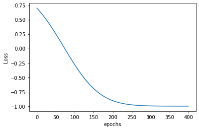
Conclusion

Note that the value of the cost function is bounded between \(-1\) and \(1\) because we take the expectation value with respect to the Pauli-Z operator. This expectation value of a state \(\psi\) with respect to \(\sigma_{z}\) is

\begin{equation} \langle \psi| \sigma_{z} |\psi\rangle \end{equation}

And it is well-known that

\begin{equation} \sigma_{z}|0\rangle = |0\rangle \\ \sigma_{z} |1\rangle = -|1\rangle \end{equation}

We see in the graph that the loss starts off bad from around \(0.75\) (when the worse it could get was \(1\)). During the optimization routine, the loss progressively gets down in \(400\) epochs to very close to \(-1\). which was the best one could expect.