Jupyter notebook implementations can be found here

Basic Qubit Rotation Example

In this example, we show how we can use a simple gradient descent method to optimize a unitary gate for qubit rotation. The idea is as follows: We start in \(|1 \rangle\) state on a Bloch Sphere and apply rotations around Z-Y-Z axes (in that order) using \(R(\phi,\theta,\omega)\), which is a general unitary operator parameterized by three real parameters, \(\phi\), \(\theta\), and \(\omega\). Each of these parameters represent the degree of rotation around x, y and z axes respectively to reach the target state, which is defined to be \(|0 \rangle\) in this case. \(R(\phi,\theta,\omega)\) has the following matrix representation:

\[\begin{split}R(\phi,\theta,\omega) = RZ(\omega)RY(\theta)RZ(\phi)= \begin{bmatrix} e^{-i(\phi+\omega)/2}\cos(\theta/2) & -e^{i(\phi-\omega)/2}\sin(\theta/2) \\ e^{-i(\phi-\omega)/2}\sin(\theta/2) & e^{i(\phi+\omega)/2}\cos(\theta/2) \end{bmatrix}\end{split}\]

import jax.numpy as jnp
from jax import grad
from jax.random import normal, PRNGKey

import numpy as onp

from qgrad.qgrad_qutip import basis, fidelity

def rot(phi, theta, omega):
    """Returns a rotation matrix represetning
    the rotation around Z-Y-Z axis.

    Parameters:
        phi (float): rotation angle for the
            first rotation around the z-axis
        theta (float): rotation angle for
            rotation around the y-axis
        omega (float): rotation angle for the
            second rotation around the z-axis

    Returns:
        :obj:`jnp.ndarray`: array representing
            the rotation matrix

    """

    cos = jnp.cos(theta / 2)
    sin = jnp.sin(theta / 2)

    return jnp.array(
        [
            [
                jnp.exp(-0.5j * (phi + omega)) * cos,
                -(jnp.exp(0.5j * (phi - omega))) * sin,
            ],
            [
                jnp.exp(-0.5j * (phi - omega)) * sin,
                jnp.exp(0.5j * (phi + omega)) * cos],
            ]
    )

def cost(phi, theta, omega, ket):
    r"""Returns the fidelity between
    the evolved state and the target
    :math:`|0 \rangle` state.

    Parameters:
        phi (float): rotation angle for the
            first rotation around the z-axis
        theta (float): rotation angle for
            rotation around the y-axis
        omega (float): rotation angle for the
            second rotation around the z-axis
        ket (:obj:`jnp.array`): Initial ket
            to act the rotation matrix on

    Returns:
        float: fidelity between the initial and
            the evolved state under rotation
    """
    evolved = jnp.dot(rot(phi, theta, omega), ket)
    return fidelity(evolved, basis(2, 0))[0][0]

Gradient Ascent Implementation

Here we have our own gradient ascent implementation. One may use traditional gradient descent by subtracting fidelity from \(1\) in the cost function.

There are multiple parameters, like epochs, alpha, etc, that one might tune further in hopes of better convergence. For our purposes, however, we see that our implementation converges well in about \(80\) crude steps.

# initialize parameters for learning
epochs = 80
alpha = 0.2  # learning rate
weights = normal(PRNGKey(0), shape=(3,))
init_ket = basis(2, 1) # initial |1> state
der_cost = grad(cost, argnums=[0, 1, 2])
state_hist = [Qobj(onp.array(init_ket))]

for epoch in range(epochs):
    der = jnp.asarray(der_cost(*weights, init_ket))
    weights = weights + alpha * der
    state_hist.append(Qobj(onp.dot(rot(*weights), init_ket)))
    fidel = cost(*weights, init_ket)
    progress = [epoch + 1, fidel]
    if epoch % 10 == 9:
        print("Epoch: {:2f} | Fidelity: {:3f}".format(*jnp.asarray(progress)))

Epoch: 10.000000 | Fidelity: 0.294945
Epoch: 20.000000 | Fidelity: 0.756419
Epoch: 30.000000 | Fidelity: 0.961341
Epoch: 40.000000 | Fidelity: 0.995116
Epoch: 50.000000 | Fidelity: 0.999403
Epoch: 60.000000 | Fidelity: 0.999927
Epoch: 70.000000 | Fidelity: 0.999991
Epoch: 80.000000 | Fidelity: 0.999999

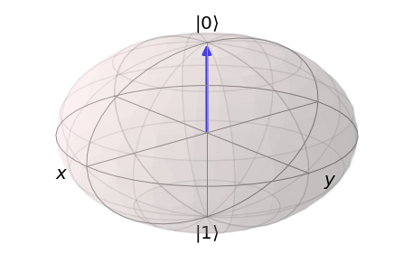
Bloch Sphere Visualization

As we see above, we started off with a very low fidelity (\(\sim\) 0.29). With gradient descent iterations, we progressively achieve better fidelities via better parameters, \(\phi\), \(\theta\), and \(\omega\). To visualize training, we render our states on to a Bloch sphere animation below.

We see how our gradient based optimizer walks from \(|1 \rangle\) (southward) and converges almost perfectly to the target state \(|0 \rangle\) (northward) as depicted in the second figure.

# Visualization
%matplotlib inline
from qutip import Bloch
from mpl_toolkits.mplot3d import Axes3D
import matplotlib.animation as animation
import matplotlib.pyplot as plt

plt.rcParams["animation.html"] = "jshtml"
fig = plt.figure()
ax = Axes3D(fig,azim=-40,elev=30)
sphere = Bloch(axes=ax)

def animate(i):
    sphere.clear()
    sphere.add_states(state_hist[i])
    sphere.make_sphere()
    return ax

def init():
    sphere.vector_color = ['b']
    return ax

ani = animation.FuncAnimation(fig, animate, onp.arange(len(state_hist)),
                            init_func=init, repeat=True)
ani

Once Loop Reflect

<Figure size 360x360 with 0 Axes>